Build stick objects from xyz (lat/long/abundance) data for use in stickplots
build_sf_sticks.RdAccepts xyz data (for example, longitude/latitude/abundance) and returns a vertical 'stick'
at each position. Sticks are returned as sf LINESTRING objects.
These objects can be plotted using ggplot2::geom_sf() or base plot.
Usage
build_sf_sticks(
  x,
  y,
  z,
  group_variable = NULL,
  return_df = NULL,
  rotation = 5,
  bar_scale = 0.5,
  crs = "EPSG:3338"
)
Arguments
- x
x- position
- y
Y- position
- z
Abundance value (the value that will be used to scale sticks)
- group_variable
If specified, will specify the group for each stick; this can be used to identify sticks by group.
- return_df
If specified, will include all columns from the original dataframe in the returned object. Only one of 'group_variable' or 'return_df' should be specified.
- rotation
Rotation of the sticks in degrees from the vertical. Default is 5 degrees. 0 = no rotation; positive values rotate bars in a clockwise direction.
- bar_scale
The relative size of sticks. Default is ~1/2 of total plot height.
- crs
The coordinate reference system (CRS) into which sticks will be projected. By default, objects will be returned using the default CRS (Albers Equal Area Alaska, EPSG 3338). Any other valid projection can be specified. Note that this relies on the sf::st_crs function- make sure you are using a valid CRS argument.
Examples
dat <- data.frame(
"x" = c(-152.2, -150.3, -159.4),
"y" = c(55.2, 55.8, 55.6),
"z" = c(7500, 40000, 28000),
"species" = c("a", "a", "b")
)
# sticks can be plotted with ggplot2::geom_sf(),
# and Coordinate Reference System (CRS) conversions are handled by sf::st_crs()
library(ggplot2)
library(sf)
#> Linking to GEOS 3.13.1, GDAL 3.10.2, PROJ 9.5.1; sf_use_s2() is TRUE
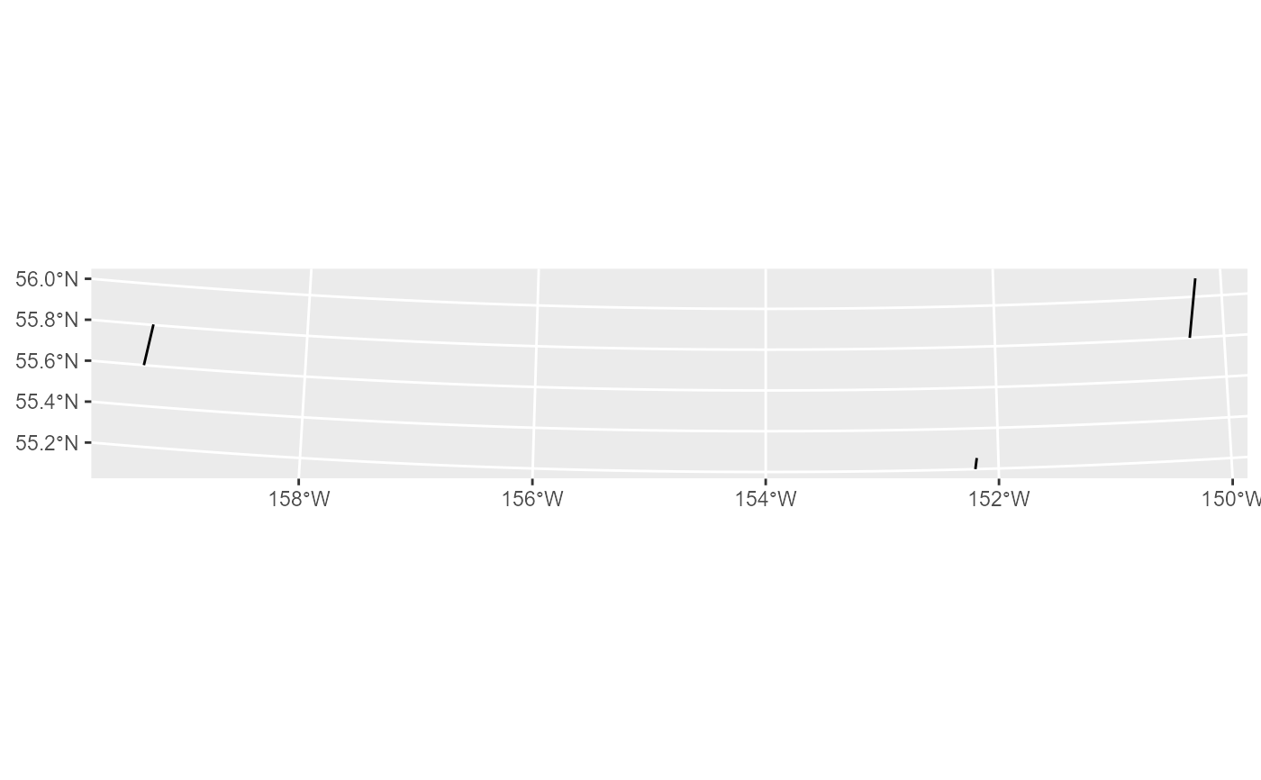
# you have to provide x,y,z at minimum
sticks <- build_sf_sticks(x = dat$x, y = dat$y, z = dat$z)
# plot with ggplot2 geom_sf()
ggplot() +
geom_sf(data = sticks)
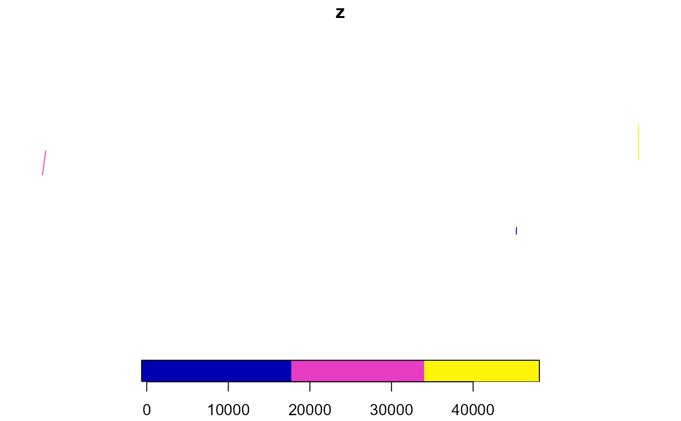
 # or with base r plotting
plot(sticks)
# or with base r plotting
plot(sticks)
 # the rotation (from 0) can be specified (in degrees from 0-360). If not specified,
# sticks will be rotated to 5 degrees
sticks <- build_sf_sticks(x = dat$x, y = dat$y, z = dat$z, rotation = 15)
ggplot() +
geom_sf(data = sticks)
# the rotation (from 0) can be specified (in degrees from 0-360). If not specified,
# sticks will be rotated to 5 degrees
sticks <- build_sf_sticks(x = dat$x, y = dat$y, z = dat$z, rotation = 15)
ggplot() +
geom_sf(data = sticks)
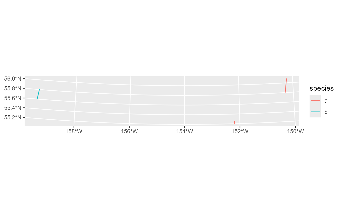
 # If a CRS is not specified, none will be assigned; if one is specified,
# it will be set using sf st_crs()
sticks <- build_sf_sticks(
x = dat$x, y = dat$y, z = dat$z, rotation = 15, crs = 3338,
group_variable = dat$species
)
ggplot() +
geom_sf(data = sticks, aes(color = species))
# If a CRS is not specified, none will be assigned; if one is specified,
# it will be set using sf st_crs()
sticks <- build_sf_sticks(
x = dat$x, y = dat$y, z = dat$z, rotation = 15, crs = 3338,
group_variable = dat$species
)
ggplot() +
geom_sf(data = sticks, aes(color = species))
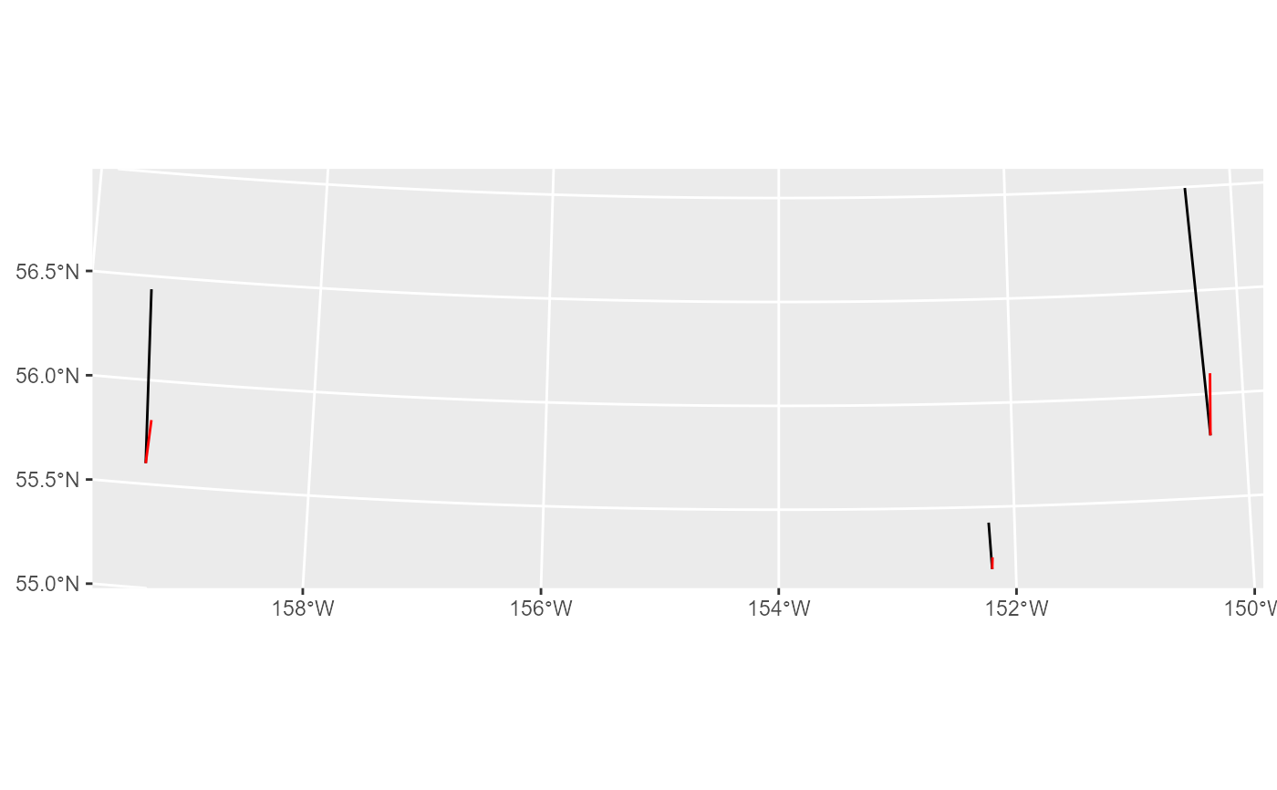
 # sticks are automatically scaled so that the largest abundance value
# this can be modified with bar_scale argument
sticks <- build_sf_sticks(x = dat$x, y = dat$y, z = dat$z, rotation = -5, bar_scale = 2)
sticks2 <- build_sf_sticks(x = dat$x, y = dat$y, z = dat$z, rotation = 5, bar_scale = .5)
ggplot() +
geom_sf(data = sticks) +
geom_sf(data = sticks2, color = "red")
# sticks are automatically scaled so that the largest abundance value
# this can be modified with bar_scale argument
sticks <- build_sf_sticks(x = dat$x, y = dat$y, z = dat$z, rotation = -5, bar_scale = 2)
sticks2 <- build_sf_sticks(x = dat$x, y = dat$y, z = dat$z, rotation = 5, bar_scale = .5)
ggplot() +
geom_sf(data = sticks) +
geom_sf(data = sticks2, color = "red")