Set your ggplot map limits a bit more easily

Returns a ggplot2 object that will limit the extent of your ggplot map to cover only the data you care about. This will be slightly larger than the extent of plot_limits_data; you can still use the param `plot_expansion` to fine-tune the plot extent.

Usage

easy_plot_limits(plot_limits_data, plot_expansion = 0.05)

Arguments

plot_limits_data

A sf spatial dataframe; this is required and used to map extent. Use the same dataframe as you used for get_basemap_layers!

plot_expansion

This controls the amount of buffer around the basemap (default is 5% (0.05) around the extent of the data; set from 0-1). This should match the value used for get_basemap_layers.

Value

a ggplot2 object that will limit the extent of your ggplot map.

Examples

library(ggplot2)
library(dplyr)
#> 
#> Attaching package: 'dplyr'
#> The following objects are masked from 'package:stats':
#> 
#>     filter, lag
#> The following objects are masked from 'package:base':
#> 
#>     intersect, setdiff, setequal, union
library(sf)
library(MACEReports)

# get some example data
dat <- data.frame(
"x" = c(-151.2, -150.3, -153.4),
"y" = c(58.2, 59.8, 56.6),
"z" = c(7500, 40000, 28000),
"species" = c("a", "a", "b"))

# create an sf dataframe
dat <- sf::st_as_sf(dat, coords = c("x", "y"), crs = 4326)

# convert CRS to a reasonable projection
dat <- sf::st_transform(dat, crs = "EPSG:3338")

# return a basemap
basemap <- get_basemap_layers(plot_limits_data = dat, bathy = FALSE)

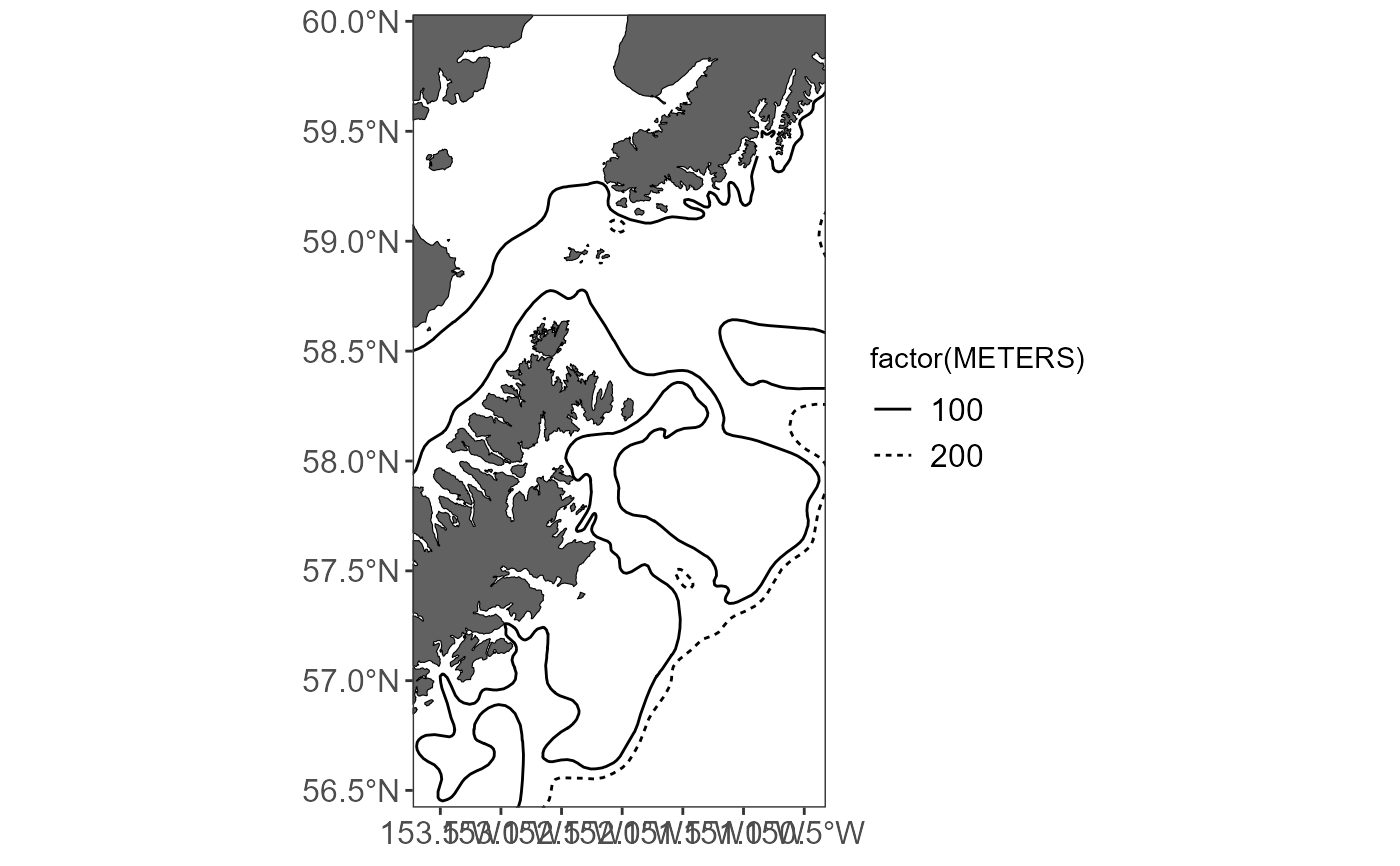
# get the bathymetry
bathy_data <- get_shapefile(shapefile_name = "alaska_bathy_contours") %>%
 filter(METERS %in% c(100,200))

# plot it
basemap +
  geom_sf(data = bathy_data, aes(linetype = factor(METERS))) +
  easy_plot_limits(plot_limits_data = dat)